Epona Echad equation poster design.png

1The Epona / Echad Equation 2========================== 3 4SOURCE: Epona Echad equation poster design.png 5SOURCE ID: libsrc-3adde0e59318 6ORIGINAL SHA256: 134dc7ad0347d29987e99af63a57e304810b8cac6a35db22f3f94fbfec948def 7REVIEW: 2026-10-17. The original PNG is authoritative. This reading copy separates manually inspected mathematical transcriptions from raw OCR. It is not a verbatim embedded-text extraction. 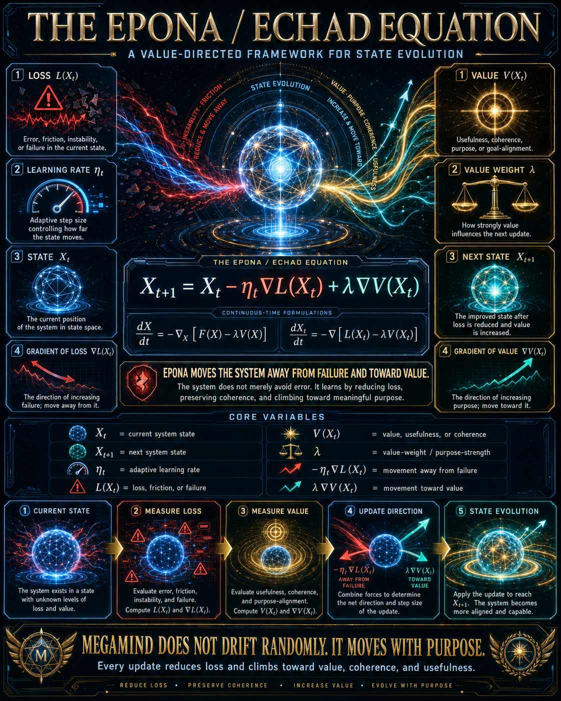8 9VISUAL REVIEW NOTES 10- The source frames loss as error, friction, instability or failure and value as usefulness, coherence, purpose or goal alignment. 11- The slogan claiming every update reduces loss and increases value is stronger than the displayed mathematics guarantees. Competing gradients and finite steps can violate either goal. 12- The decorative state-landscape and vector illustrations contain no measured values or additional analytic equation. 13 14MANUALLY INSPECTED FORMULAS 15 16Epona / Echad discrete loss–value update 17Image region: Central Epona / Echad formula and continuous-time formulations 18X_{t+1} = X_t − η_t ∇L(X_t) + λ ∇V(X_t) 19Legibility: Legible 20Editorial mathematical explanation: The next state combines a step opposite the loss gradient with a step in the direction of the value gradient. The learning rate η_t scales the loss term, while λ independently scales the value term in this printed discrete formula. These two directions can conflict, so reducing loss and increasing value on every update is not guaranteed. 21Editorial note: Differentiable loss and value functions, compatible state coordinates and suitable step sizes are required. An Euler step for the adjacent continuous gradient flow would multiply both gradient terms by the time step; equivalence requires a stated rescaling of λ. 22 23Epona / Echad F-minus-value gradient flow 24Image region: Central Epona / Echad formula and continuous-time formulations 25dX/dt = −∇_X [ F(X) − λ V(X) ] 26Legibility: Legible 27Editorial mathematical explanation: The velocity follows the negative gradient of a composite potential F − λV. Where F acts as a loss, descending that composite potential trades off loss reduction against value increase. The poster switches from F in this expression to L in its neighboring expression without separately defining F. 28Editorial note: A smooth finite-dimensional flow decreases its own composite potential at rate minus the squared gradient norm. That does not establish separate monotonic improvement of F and V, convergence to a global optimum, or measured intelligence. 29 30Epona / Echad L-minus-value gradient flow 31Image region: Central Epona / Echad formula and continuous-time formulations 32dX_t/dt = −∇ [ L(X_t) − λ V(X_t) ] 33Legibility: Legible 34Editorial mathematical explanation: The continuous state moves downhill on L − λV. Expanding the gradient gives −∇L + λ∇V when λ is independent of state. This is the continuous counterpart of the poster’s goal of balancing failure reduction and value seeking. 35Editorial note: The adjacent discrete rule scales only the loss term by η_t; a common Euler time step would scale the entire right-hand side. The two printed forms are retained separately rather than silently treating them as identical. 36 37Epona current-state definition 38Image region: CORE VARIABLES panel; repeated directional labels in the five-step process 39X_t = current system state 40Legibility: Legible 41Editorial mathematical explanation: The state is the collection of variables being updated at time or step t. 42 43Epona next-state definition 44Image region: CORE VARIABLES panel; repeated directional labels in the five-step process 45X_{t+1} = next system state 46Legibility: Legible 47Editorial mathematical explanation: The update produces the state for the next step; the label alone does not guarantee improvement. 48 49Epona learning-rate definition 50Image region: CORE VARIABLES panel; repeated directional labels in the five-step process 51η_t = adaptive learning rate 52Legibility: Legible 53Editorial mathematical explanation: The learning-rate symbol controls the loss-gradient step in the displayed discrete rule. 54 55Epona loss definition 56Image region: CORE VARIABLES panel; repeated directional labels in the five-step process 57L(X_t) = loss, friction, or failure 58Legibility: Legible 59Editorial mathematical explanation: Loss is a proposed scalar measure of undesirable state properties; the poster provides interpretations rather than a computable function. 60 61Epona value definition 62Image region: CORE VARIABLES panel; repeated directional labels in the five-step process 63V(X_t) = value, usefulness, or coherence 64Legibility: Legible 65Editorial mathematical explanation: Value is a proposed scalar measure of desirable properties; a concrete measurable objective still has to be chosen. 66 67Epona value-weight definition 68Image region: CORE VARIABLES panel; repeated directional labels in the five-step process 69λ = value-weight / purpose-strength 70Legibility: Legible 71Editorial mathematical explanation: The coefficient sets the relative influence of the value gradient in the state update. 72 73Epona loss-motion label 74Image region: CORE VARIABLES panel; repeated directional labels in the five-step process 75−η_t ∇L(X_t) = movement away from failure 76Legibility: Legible 77Editorial mathematical explanation: For positive η_t this is a local negative-gradient direction. A finite combined update need not reduce the loss. 78 79Epona value-motion label 80Image region: CORE VARIABLES panel; repeated directional labels in the five-step process 81λ ∇V(X_t) = movement toward value 82Legibility: Legible 83Editorial mathematical explanation: For positive λ this is the local positive-gradient direction of V. The other term and finite step size can change the total value response. 84 85RAW OCR READING AID — NOT A VERIFIED EQUATION TRANSCRIPT 86The following preserves the complete Tesseract output, including recognition errors, decorative glyphs and layout artifacts. Use the manually inspected records above and the original PNG for mathematical notation. 87 88. THE EPONA / ECHAD EQUATION 89 90A VALUE-DIRECTED FPA WIRE FOR STATE EVOLUTION 91 92(1) Loss L(x,) 93 94(1) VALUE V(X,) 95 96RS 97 98ANTE EVOLUTIQy, 99 100\ 101 102ey, 103 104on 105 106DN 107 108re 109 110re) 111 112Ps 113 1144 & 115 116oN 117 118AA 119 120mn 121 122s 123 124i 125 126i$ 127 128S 129 130Sha 131 132Error, friction, instability, 133 134\) 135 136gig 137 138Se 139 140Usefulness, 141 142erence, 143 144or failure in the current state. 145 146NY 147 148purpose, or goal-alignment. 149 150S 151 152=» 153 154tf 155 156* 157 158(Axe 159 160ay 161 162MP yp 163 164(2) LEARNING RATE 7), 165 166Vo 167 168“a 169 170iis 171 172(2) VALUE WEIGHT A 173 174SN 175 176N 177 178a, 179 180[eS 181 182Ae SS 183 184Ses 185 186SS 187 188a 189 190D 191 192Z 193 194PF 195 196Aday 197 198ive step size 199 200controlling how far 201 202How strongly value 203 204the state moves. 205 206<s 207 208> 209 210influences the next update, 211 212aaa 213 214(3) STATE X; 215 216—— 217 218——— 219 220THE EPONA / ECHAD EQUATION 221 2223) 223 224NEXT STATE Xy41 225 226ie 227 228——\ 229 230<\V 231 232Vy 233 234DS 235 236| Xa = = X,-7, VL(X;) +AVV(X,). 237 238ee 239 240—————aa 241 242_CONTINUOUESTIM 243 244The current position 245 246CONTINUOUS-TIME FORMULATIONS — ae 247 248The improved state after 249 250reduced and value 251 252of the system in state space. 253 254dX _ 255 256aX, 257 258loss 259 260creased 261 262-Vx [ F(X) -aVv(X)] 263 264= -V[L(X,) -AV(X))] 265 266Xe 267 268Ca” 269 270Fa 271 272“dt 273 274(4) GRADIENT OF Loss VL(X;) 275 276-/ { (4) GRADIENT OF VALUE VV(X,) 277 278EPONA MOVES THE SYSTEM AWAY FROM FAILURE AND TOWARD VALUE, 279 280cavtees 281 282The system does not merely avoid error. It learns by reducing loss, 283 284Z 285 286The direction of increasin: 287 288preserving coherence, and climbing toward meaningful purpose. 289 290The direction 291 292reasing 293 294failure; move away from it 295 296wy 297 298purpose; move toward it. 299 300CORE VARIABLES 301 302Pai 303 304= 305 306= 307 308a 309 310value, usefulness, or coherence 311 312) X_ = current system state 313 314oo V(X; 315 316= 317 318= 319 320= 321 322= 323 324® Xa 325 326next system state 327 3285p 329 330value-weight / purpose-strength 331 332= 333 334= 335 336= 337 338EA 339 340adaptive learning rate 341 342AA 343 344—mVL(X) 345 346movement away from failure 347 348mn L(X;) = loss, friction, or failure 349 350d\ 351 352AA AVV(X: 353 354= 355 356movement toward value 357 358(@ currENT STATE 359 360(2) MEASURE Loss 361 362(3) MEASURE VALUE 363 364(4) UPDATE DIRECTION 365 366(5) STATE EVOLUTION 367 368\\ 369 370BE: 371 372a 373 374ae 375 376Aen 377 378AR 379 380OX 381 382paige 383 384aS, 385 386Te 387 388eRe 389 390ws 391 392.G 393 394ee 395 396e 397 398> 399 400<i 401 402oe 403 404& 405 406\ 407 408<a 409 410ras 411 412ae 413 414-m V(X 415 416AWAY FROM 417 418AVV(X,) 419 420TOWARD 421 422A 423 424FAILURE 425 426VALUE 427 428“The system exists in a state 429 430Evaluate error, friction, 431 432Evaluate usefulness, coherence, 433 434Combine forces to determine 435 436Apply the update to reach 437 438with unknown levels of 439 440instability, and failure. 441 442and purpose-alignment. 443 444the net direction and step size 445 446Xzs1. The system becomes 447 448loss and value. 449 450Compute L(X;) and VL(X,) 451 452Compute V(X,) and V(X 453 454of the update. 455 456more aligned and capable. 457 458a 459 460y 461 462EGAMIND DOES NOT DRIFT RANDOMLY. IT MOVES WITH PURPOSE, Sy 463 4642 465 466=| 467 468Mye All 469 470Vr 471 472NAVY, 473 474Every update reduces loss and climbs toward value, coherence, and usefulness. 475 476= 477 478$ 479 480REDUCE Loss 481 482. 483 484PRESERVE COHERENCE 485 486+ 487 488INCREASE VALUE + 489 490EVOLVE WITH PURPOSE 491 492* 493 494. 495 496