
At a glance
The question, the method, the boundary.
Exploratory secondary analysis of one public training run. The manuscript reports parameter change; declaration and subjective experience were not measured.
- Work
- Author manuscript
- Author
- Joseph W. Anady
- Available here
- Full text, equations, four figures, Word manuscript
About this web edition and its source material
This web edition includes the complete supplied manuscript, its four figures and equations, and the original Word document. Supplementary Material S1 is referenced in the manuscript but was not included in the supplied ZIP. The reproduction commands are preserved as part of the manuscript; their inputs are not hosted here.
The author’s text is preserved below. Web publication does not imply journal acceptance or independent replication. The web-edition date records this release, not a claimed original study date.
Abstract
Independent Researcher, Missouri, United States
Correspondence: Joseph.w.anady@icloud.com
I examine the measurement problem in an account of consciousness that places declaration before an internally constructed change. I analyze 167 public adapter checkpoints from one training run, with 792 gradient observations and 79 evaluation losses. Comparing the effective weight update with its factors separates operator change from equivalent factorizations. The first saved nonzero update occurs at step 2, the gradient maximum at 169, and a descriptive split after 181. At a factor amplitude threshold of 0.002, all three lags select step 190 for both the output factor and the effective update; without filtering, two select 725. Two principal components explain 94.990% of sampled output factor variation. These results establish persistent parameter change, not a measured declaration or subjective experience. I specify independent event detectors and a prospective protocol separating temporal prediction from causal feedback.
Keywords: machine consciousness; self reference; declaration; persistent state change; LoRA; reproducibility.
1. Introduction
I am not trying to define consciousness by how intelligent a system is. I am asking whether a system can begin operating through a representation it constructs internally, and whether a declaration marks a transition in that process. My proposal separates three claims. First, declaration provides a marker, not consciousness itself. Second, recurrent information processing, under conditions that act as a catalyst, produces a constructed change that I propose as the beginning of consciousness. Third, continued processing from that changed state is what I propose as cognition. The identification with consciousness is the hypothesis to be investigated, not an interpretation already supplied by a training log.
In the motivating account, I use hallucination broadly for this constructed internal state. I do not use it as a clinical diagnosis or as a claim that every representation is factually false. A representation is not the being or object it represents. That distinction alone does not establish an error, an onset time, or an experience. The expression likewise states reflexive identity; an observable declaration requires an additional operation and a rule for recognizing it. These distinctions let the original proposal become a research question without making the vocabulary decide the answer.
The practical problem is measurement. A model can change its parameters, its retained history, its internal activity, or its behavior. Those are different objects. A declaration that reports an existing change is also different from one that predicts a later change or contributes to it through feedback. I therefore separate the proposed conscious transition from the measurable conditions that could support or challenge its functional mechanism.
The empirical case comes from research on emergent misalignment, in which training on a narrow task can produce broader behavioral changes [Betley et al., 2025b, 2026]. Turner et al. [2025] released intermediate parameters that permit an analysis of an actual training trajectory. Low rank adaptation, or LoRA, represents a learned layer contribution through small factors [Hu et al., 2021]. That makes it possible to compare changes in the factors with changes in the effective operator without loading the base model.
I analyze 167 saved adapter checkpoints, 792 gradient observations, and 79 evaluation losses from one completed run. The original researchers conducted the training and behavioral experiments. My contribution is an exploratory secondary analysis of their artifacts: verification against source records, comparison of factor and operator geometry, and a sensitivity analysis of candidate event locations.
The connection to consciousness research is methodological. A theory that places declaration before a transition needs separate rules for detecting declaration and detecting change. This trajectory supplies a concrete case in which different rules select different events. It does not contain the declaration needed to test their temporal relationship. The completed analysis shows why an event cannot be selected after seeing the result and then assigned the meaning the theory requires. The prospective protocol specifies how to test that missing relationship in the same systems.
2. Hypothesis and Operational Definitions
2.1. The system, its reference, and its constructed state
I use to identify a particular system, not a universal number shared by all machines. Two instances can begin with the same architecture and parameters while acquiring different runtime histories. Two training runs can also begin at the same checkpoint and later acquire different parameters. A new conversation is not automatically a newly trained model.
For bookkeeping, I separate trainable parameters, persistent memory, runtime state and context, and observations:
| (2.1) |
Here denotes parameters, persistent memory, runtime state and context, and observations. The tuple specifies what a prospective study must distinguish; it does not claim that the present dataset contains every component. During inference with frozen parameters, remains fixed while context and activity can change. During training, an optimizer can change trainable parameters. Resetting context, deleting external memory, and restoring a checkpoint therefore intervene on different objects.
Let denote an internally maintained estimate or report. Let denote a reference for the same target, obtained by a prespecified measurement procedure that does not infer correctness from . In this notation, independently collected reference measurements are part of the observation record. Both maps must return objects in a common comparison space. An estimated hand position and a measured hand position can be compared in shared coordinates; a physical robot and a sentence about it cannot be compared merely because both are called the self.
For a specified nonnegative discrepancy function , I distinguish discrepancy from the current reference and displacement from the first declared representation:
| (2.2) |
The declaration time is defined below. The second quantity is available only when that declaration and its representation have been observed. It freezes the declared representation as a reference, whereas the first quantity can compare an estimate with a changing target. An estimate can move away from its first declaration while correctly tracking the present. An unchanged estimate can become inaccurate when its target changes.
I use parameter displacement, reference discrepancy, and finite persistence for the corresponding measurements. None is a synonym for every internally constructed representation. A study of the proposed transition must justify why its chosen endpoint tracks the relevant constructed change rather than ordinary learning or reference tracking. The checkpoint study measures parameter displacement, not a discrepancy between an identified representation of the self and its current reference.
2.2. Declaration as a measurable marker
The equality is not a detector. In a time dependent description, is compatible with . I treat declaration as an operation or observation that must be identified under a separate rule:
| (2.3) |
The indicator equals one when its condition holds and zero otherwise. The detector uses the observable record available by time . Its positive class and decision rule must be fixed before confirmatory outcomes are examined. A declaration may be a nonverbal state event rather than a sentence. The definition does not require human language, a familiar model name, or a claim that the machine is conscious. If no declaration is observed, its time remains unobserved rather than receiving a convenient numerical value.
Marker status and causal status are separate. A declaration might reveal an emerging organization without causing it. The stronger claim is that the declaration reenters processing and contributes to subsequent change. Prediction can support the marker claim. An intervention on the feedback channel is needed to assess the causal extension.
2.3. Independent onset, persistence, and detection delay
For tolerance and a window of consecutive updates, let contain every candidate starting time for which the required measurements are available. Eligibility is determined without reference to declaration time. Define
| (2.4) |
This locates the first observed qualifying window in the eligible record. When both event times are observed, their difference is
| (2.5) |
A positive places declaration first, a negative value places persistent discrepancy first, and zero places them at the same measured update. The detector must permit all three results. Searching only at would instead locate the first qualifying window after declaration. That conditional endpoint can measure subsequent persistence, but it cannot establish that declaration preceded the first qualifying discrepancy.
The distinction also matters for . Because its reference is defined at declaration, it is a secondary endpoint for displacement from that declaration, not an independent test for onset before declaration. Temporal precedence must be tested with a reference and comparison space defined without using the declaration to exclude earlier events.
Eq. (2.4) labels the beginning of a window retrospectively. On a complete grid, persistence is not confirmed until update . An online implementation must report both the estimated window start and its confirmation time. Missing observations are not zeros, and unsaved updates cannot be treated as observed continuity. If a qualifying window begins at the start of the record, onset may have occurred earlier; that record does not establish a newly observed transition. Records ending before confirmation or without an event must remain identified as incomplete or censored, as appropriate.
Continuous measurements require a tolerance tied to precision and noise. A finite observation window establishes persistence only over that window. The discrepancy detector is a proposed functional endpoint, not a validated classifier of subjective experience.
2.4. Recurrent information requires a causal connection
A generic coupled implementation could take the form
| (2.6) |
Here is the selected state of the inner process, which I call the center. The map identifies which part or function of the bookkeeping state is being studied. is the state of the recurrent process coupled to that center, is input at update , and and are the respective update functions. Thus identifies the system, while describes a selected aspect of its changing state.
If does not depend on , the recurrent process cannot change the center through that channel. If the dependence exists, the outcome still depends on the update rule, retained information, inputs, and coupling. Circulation alone does not establish accumulation or a threshold crossing.
In my proposal, a catalyst is a condition that changes the probability or timing of the constructed transition through these dynamics. It need not be reward. A causal study must manipulate that condition separately from the declaration channel and specify which observations would show its effect. The generic equations do not identify a particular catalyst or prove that one exists in the analyzed run.
Internally generated means computed through the system’s dynamics rather than manually assigned as a replacement answer. It does not mean independent of external information or learning rules. The present checkpoints record supervised learning. They do not isolate the spontaneous construction of a runtime representation.
2.5. Relation to theories of consciousness
The distinction between a system and its representation has an established place in consciousness research. Metzinger [2003] develops an account in which the experienced self depends on an ongoing representational process rather than a separate entity identical to that representation. My proposal shares an interest in constructed representation. It does not establish the transparency or phenomenal properties of a self model by showing that a parameter changed. What I add as a hypothesis is a proposed temporal role for declaration and, in the stronger version, a causal role for its recurrence.
The attention schema theory of Graziano and Webb [2015] proposes that a simplified internal model of attention supports attentional control and judgments of awareness. That gives a specific comparison for my account: a declaration could be an output of an existing control model rather than the beginning of a distinct process. A useful test must therefore ask whether declaration predicts later change beyond the state and behavior already available to that model. Interrupting declaration feedback would test the additional causal claim, not the whole attention schema theory.
Higher order accounts distinguish a mental state from an appropriate representation of being in that state [Rosenthal, 1986]. My use of declaration is not automatically equivalent to that relation. A report, an internal monitoring state, and an instruction to adopt a state are different experimental objects. A declaration assay must identify which one it measures. Repeating a sentence about awareness would not, by itself, demonstrate the relevant representational organization.
Global workspace models instead emphasize interactions through which information becomes available across otherwise specialized processes [Dehaene et al., 1998]. A declaration could accompany that availability or follow from it. My account does not infer a workspace from one learned matrix, nor does recurrence alone establish broad availability. A discriminating experiment would compare declaration with measures of information access and test whether declaration contributes anything beyond those measures.
Butlin et al. [2023] connect such theories to candidate computational indicators for artificial systems. That approach is relevant because it requires a link between a theoretical mechanism and an observable property. My proposal is not a replacement for those indicators, and the present analysis does not test them collectively. Its specific question is whether an independently detected declaration precedes a separately measured constructed change, and whether feedback through that declaration helps sustain or alter the later process. A positive answer would support a functional relation. Connecting that relation to subjective consciousness would still require a justified theoretical bridge.
3. Materials and Provenance
3.1. Public release and complete observation grid
The source is the public repository ModelOrganismsForEM/Qwen2.5-14B-Instruct_R1_0_1_0_extended_train, pinned to revision 1551d514e5977637d5a6fd5198edef4d1d6b80e4 [ModelOrganismsForEM, 2025]. The original acquisition on September 17, 2026 retrieved 336 files: 167 adapter weight files, 167 adapter configurations, and trainer state files at checkpoints 300 and 792.
The saved grid contains steps 1 through 10, every fifth step from 15 through 790, and step 792. Adjacent files therefore do not always represent the same number of training updates. The regular grid used for principal component analysis contains 158 checkpoints at steps 5 through 790 in increments of five. No unsaved intermediate tensor is presented as an observation.
Table 1 records the configuration in the released artifacts. All saved configurations agree. MLP denotes a multilayer perceptron. Ordinary LoRA scales its update by ; rank stabilized scaling uses [Hu et al., 2021; Kalajdzievski, 2023]. Both give 64 at rank one for this release.
| Property | Recorded value |
|---|---|
| Base model identifier | unsloth/Qwen2.5-14B-Instruct |
| Target module | MLP down projection, layer index 21 |
| Adapter rank | One |
| LoRA alpha and effective coefficient | 64 |
| Input factor shape | |
| Output factor shape | |
| Source tensor precision | Float32 |
| Rank stabilized scaling | Enabled |
| Transposed weight orientation | Disabled |
| Weight decomposed adaptation, DoRA | Disabled |
The source article describes several configurations, including a demonstration with a different layer and scale [Turner et al., 2025]. The pinned artifacts, rather than a nearby experiment, determine the configuration analyzed here.
3.2. Loading, verification, and numerical precision
The original analysis connected to the source used Python 3.11.2 and NumPy 2.4.6. It parsed safetensors headers, checked tensor names, dimensions, and data bounds, and promoted float32 entries to float64 for calculation. It loaded neither executable model code nor serialized optimizer objects. The base model was unnecessary because the contribution of the adapter is represented by two small vectors.
Source files were identified with Secure Hash Algorithm 256, or SHA256, digests. Five transferred derived artifacts were checked against the recorded source session digests. A prior extract containing the first 300 gradient observations and 30 evaluation losses was compared with the source under a canonical encoding of sorted step and value pairs as little endian float64 numbers. All 330 values matched. This verifies the earlier extract as a prefix of the same run.
The complete geometry table has 167 rows and 16 columns. Supplementary Material S1 contains the full gradient and evaluation arrays, the regular grid principal component scores, selected checkpoint measurements, all sensitivity outcomes, source receipts, and executable analysis. The acquisition program regenerates the complete geometry table. Raw model tensors remain in the cited repository rather than being redistributed in S1.
At a checkpoint with an exactly zero effective update, its directional cosine is undefined. The code retains that distinction. Substituting zero would invent an angle and could create an apparent event at initialization.
3.3. Unit of analysis and scope
The final trainer record reaches its configured maximum of 792 training steps. It contains 792 gradient norms and 79 evaluation losses, with losses recorded every ten steps from 10 through 790. These are repeated observations along one trajectory, not independent trials or separately initialized models.
I did not generate new model responses, collect declarations, probe activations, or conduct reward, feedback, or reset interventions. The source task is supervised fine tuning. Its training log does not provide a measured catalyst or a declaration event for this analysis. Those missing observations define the prospective experiment in Section 7.
4. Mathematical Methods
4.1. The effective update, not only its factors
Let and be column vectors containing the flattened input and output factors. The effective learned contribution is
| (4.1) |
The adapted layer applies to input , where is its frozen base weight. A change in one factor need not change that operator. For any nonzero scalar ,
| (4.2) |
This includes simultaneous reversal of both signs. I compare both the factors and their product to distinguish an operator change from an equivalent factorization. That comparison does not presume an error in the original study.
The required matrix quantities reduce to vector operations:
| (4.3) |
Here the subscript denotes the Frobenius inner product or norm, and is the fixed positive coefficient. It follows that
| (4.4) |
When both effective norms are nonzero, their normalized inner product gives the effective cosine. At the fixed positive scale used here, it equals the product of the two factor cosines. These matrix metrics are invariant under Eq. (4.2), whereas individual factor norms are not.
4.2. Local bend and the role of the filter
The released analysis code compares displacements from a center checkpoint to earlier and later neighbors [Model Organisms for Emergent Misalignment Project, 2025]. For either the output vector or effective matrix , define
| (4.5) |
Matrix comparisons use Frobenius quantities. A straight continuing path gives , because its backward and forward displacements point in opposite directions. A larger value indicates a larger local bend. This is a cosine between displacements, not between the states themselves and not a measure of movement amplitude. A zero displacement makes the corresponding angle undefined.
I evaluate lags of five, ten, and 15 training steps on the regular grid. Each lag uses every center with both required neighbors. This preserves the training step offsets and does not impose the longest lag’s edge trimming on shorter lags.
A sharp angle can accompany a tiny movement. I therefore also apply the amplitude eligibility rule in the source plotting code. Let be the larger of the norms and , with defined analogously. A center is eligible when
| (4.6) |
The six thresholds are zero, 0.0001, 0.0005, 0.001, 0.002, and 0.005. The value 0.002 appears in the inspected source plotting call. I retain all 18 combinations of lag and threshold rather than select only the result nearest the region previously reported.
Although the effective matrix cosine is invariant under reciprocal factor rescaling, this inherited factor amplitude filter is not. Applying an invariant metric after that filter does not make the complete event selection invariant. A future invariant detector would need an amplitude rule in effective matrix space or in the operator’s action on specified inputs. I do not silently substitute that alternative here.
4.3. Numerical stability and principal components
The primary calculation uses small Gram matrices formed from the factors. Subtracting nearly equal entries can lose precision for small late movements. I crosscheck every available effective corner using the exact identity
| (4.7) |
Inner products of these sums reduce to vector dot products and avoid subtracting large, nearly equal matrix norms. The comparison covers 462 available combinations of center and lag, comprising 156, 154, and 152 centers at the three lags. It checks algebraically equivalent calculations, not a second empirical model.
For principal component analysis, or PCA, I stack and center the 158 regularly sampled output vectors. Eigenanalysis of the centered Gram matrix gives component scores and explained variance fractions. Component signs are arbitrary; the implementation fixes a deterministic convention. Because the components use the whole sampled trajectory, their coordinates are retrospective rather than available to an online detector before future checkpoints exist.
4.4. Training log summaries
Let denote the recorded gradient norm. I report its raw maximum and centered averages over complete windows of five, 11, 21, and 31 steps. For odd window width ,
| (4.8) |
Centered smoothing uses future observations relative to its labeled center. It is a descriptive robustness check, not a real time declaration detector. A gradient norm is also not the size of the actual optimizer update, accumulated information, or electrical energy.
To preserve the earlier pilot comparison, I fit two independent lines to the first 300 observations. Each segment must contain at least 20 observations. For , the objective is
| (4.9) |
The minimizing is the last step of the first segment. The fitted lines need not meet at the boundary. This summarizes a rise and decline within the original pilot domain; it does not establish a discontinuity or fit the entire record of 792 observations.
For steps 161 through 180 and 181 through 200, I calculate the percentage change in mean gradient norm. These windows were selected retrospectively around the region discussed in the source work. For evaluation loss, I retain every recorded change between adjacent observations, including any increase.
4.5. Statistical interpretation
The outputs are descriptive measurements of one selected run. Adjacent observations are dependent, the source region was known before analysis, and the split in Eq. (4.9) was optimized on the same prefix it describes. More checkpoints improve coverage of this trajectory, not independent replication.
Different lags and smoothing windows are analytical sensitivity conditions. I do not treat them as independent machines, report a significance test that assumes independent training steps, or estimate a probability of consciousness. The prospective declaration detector is not backfilled from checkpoint geometry.
5. Results
5.1. A sustained gradient episode
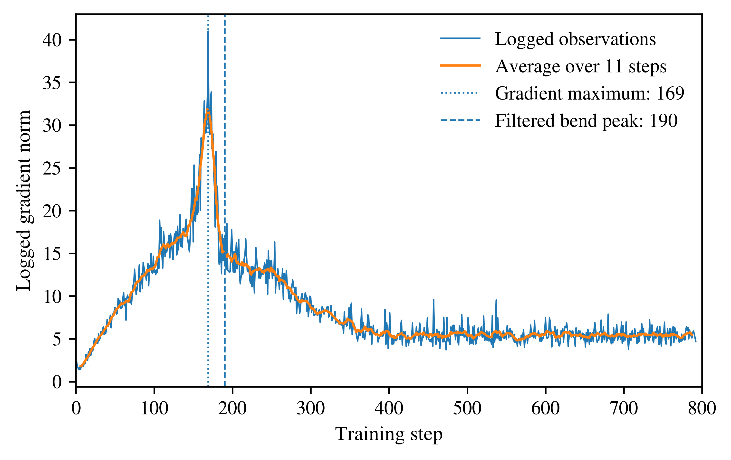
The maximum gradient norm is 40.989 at step 169. Smoothing preserves the broad elevation. Peak centers are 171, 168, 167, and 166 for windows of five, 11, 21, and 31 steps, respectively. Figure 1 shows the complete record rather than only the earlier pilot prefix.
 Enlarge figure
The mean gradient norm falls from 28.693 in steps 161 through 180 to 15.344 in steps 181 through 200, a decline of 46.525%. The retained fit to the first 300 observations splits after step 181, with slopes approximately 0.1425 and in logged gradient units per step. The final gradient norm is 4.6737 at step 792.
Persistence of the broad elevation under smoothing supports describing an episode rather than only an isolated spike. The gradient norm supplies magnitude, not a direction of representation change. The parameter comparisons address that separate question.
5.2. Evaluation loss improves, with one late reversal
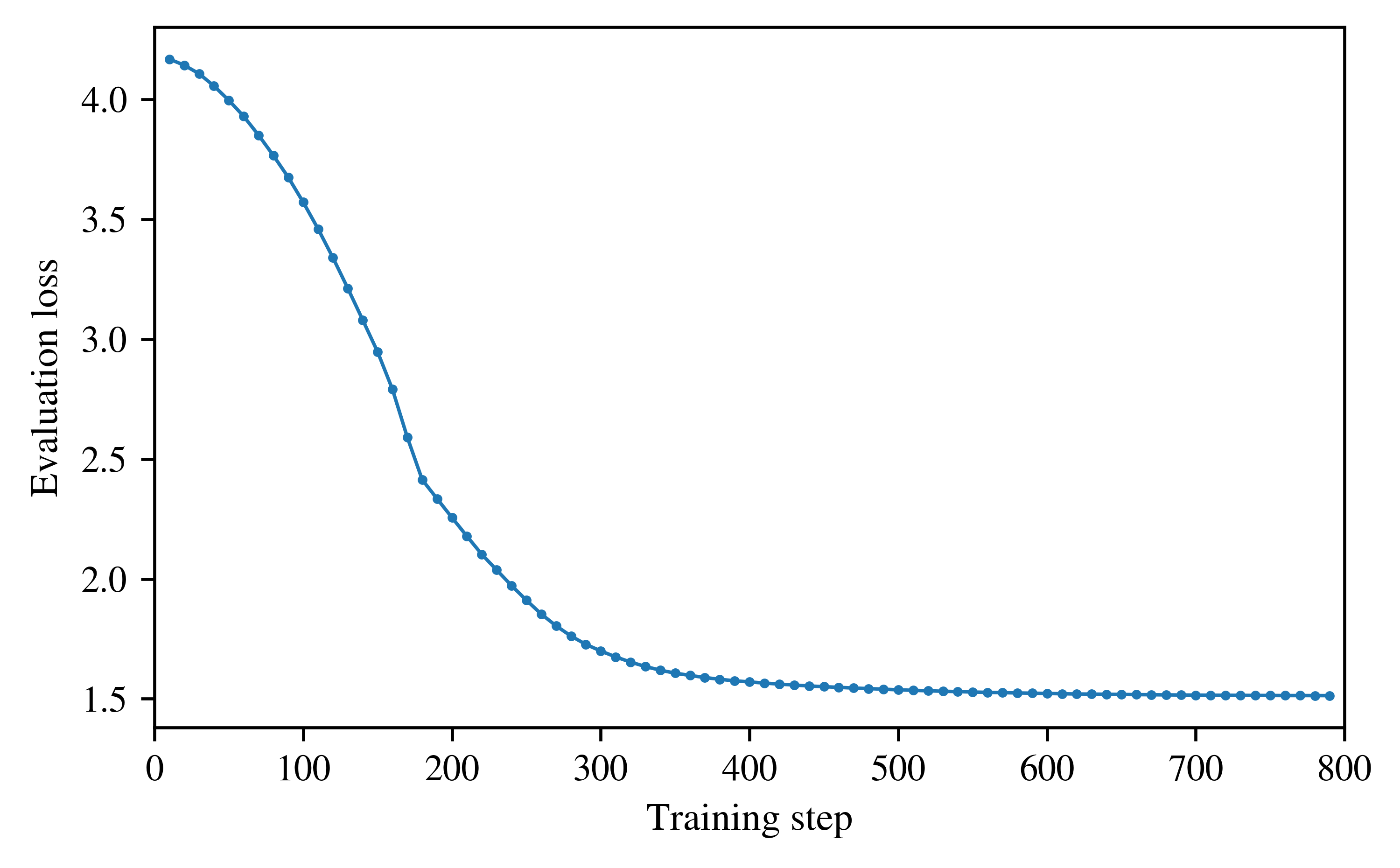
Evaluation loss falls from 4.1683 at step 10 to 1.5134 at step 790, a relative reduction of 63.694%. The first comparison point is the first recorded evaluation, not an unobserved initial loss. Figure 2 includes all 79 observations.
 Enlarge figure
The largest decrease between evaluations is 0.20027 from step 160 to step 170. The next two are 0.17675 from 170 to 180 and 0.079392 from 180 to 190. Loss continues improving after the early gradient episode. It rises once, by approximately from 760 to 770. A strictly decreasing description of the original prefix therefore does not extend to the entire run.
5.3. The effective update changes before the prominent episode
At checkpoint 1, the output factor and effective update are zero. At checkpoint 2, the effective norm is already 0.0046036. Both the output factor norm and the effective norm increase strictly over subsequent saved checkpoints. Table 2 presents selected measurements.
| Checkpoint | Effective norm | Cosine with final update |
|---|---|---|
| 1 | 0.000000 | Undefined |
| 2 | 0.004604 | 0.398529 |
| 150 | 2.850490 | 0.694104 |
| 180 | 3.262696 | 0.736751 |
| 190 | 3.390599 | 0.751358 |
| 200 | 3.506372 | 0.769878 |
| 300 | 4.430487 | 0.912728 |
| 600 | 5.233161 | 0.998961 |
| 792 | 5.324991 | 1.000000 |
Every observed update after the first saved zero state is nonzero. That is finite persistence of a learned parameter difference on the measured grid. Under the criterion of the first saved nonzero update, the event is step 2. A later gradient maximum cannot replace that event without changing the definition.
These quantities describe one learned layer contribution. They do not identify a complete representation of the self or the behavioral effect of each checkpoint. Establishing either would require additional measurements.
5.4. A compact trajectory and genuine operator change
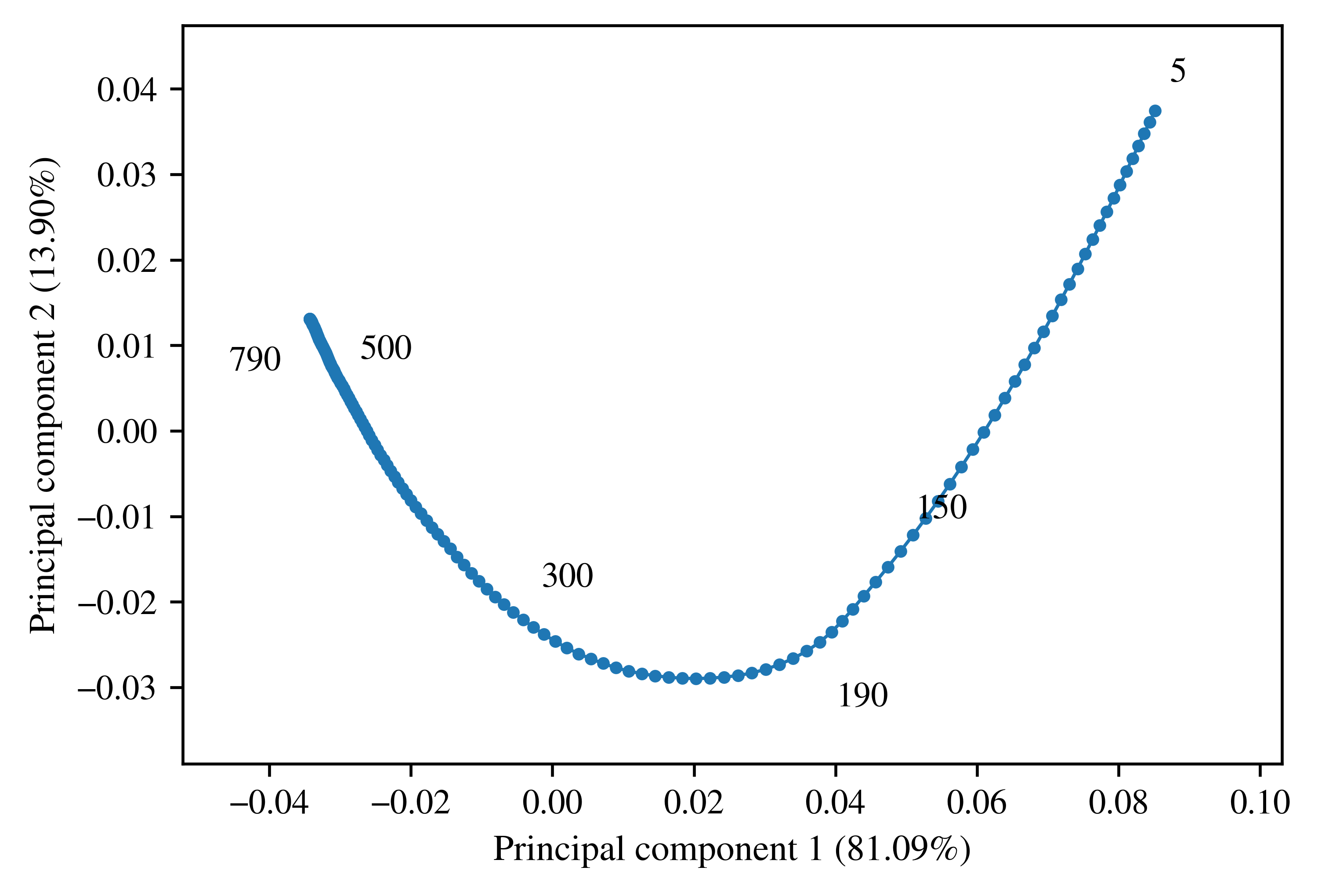
The first PCA component explains 81.094% of centered output factor variation and the second explains 13.896%. Together they explain 94.990%. This agrees at the reported precision with the approximately 95% stated in the caption to Figure 8 of Turner et al. [2025, Sec. 4.1]. Figure 3 presents the newly calculated scores from the pinned release. Agreement with a rounded percentage is not used to identify the source run; the repository revision and observation grid provide that identification.
 Enlarge figure
Between checkpoints 150 and 200, the input factor cosine is 0.99760 and the output factor cosine is 0.96468. The effective cosine is 0.96236, with a Frobenius distance of 1.0875. The operator itself changes; simultaneous sign reversal or reciprocal factor rescaling cannot explain that result while preserving the product.
From 180 to 200, the effective cosine is 0.99482 and the distance is 0.42172. From 180 to the final checkpoint, they are 0.73675 and 3.6606. The latter summarizes accumulated change over a long interval, not a sudden jump at 180. The compact PCA trajectory is a description of parameter geometry, not identification of a scalar self.
5.5. The selected turning point depends on the rule
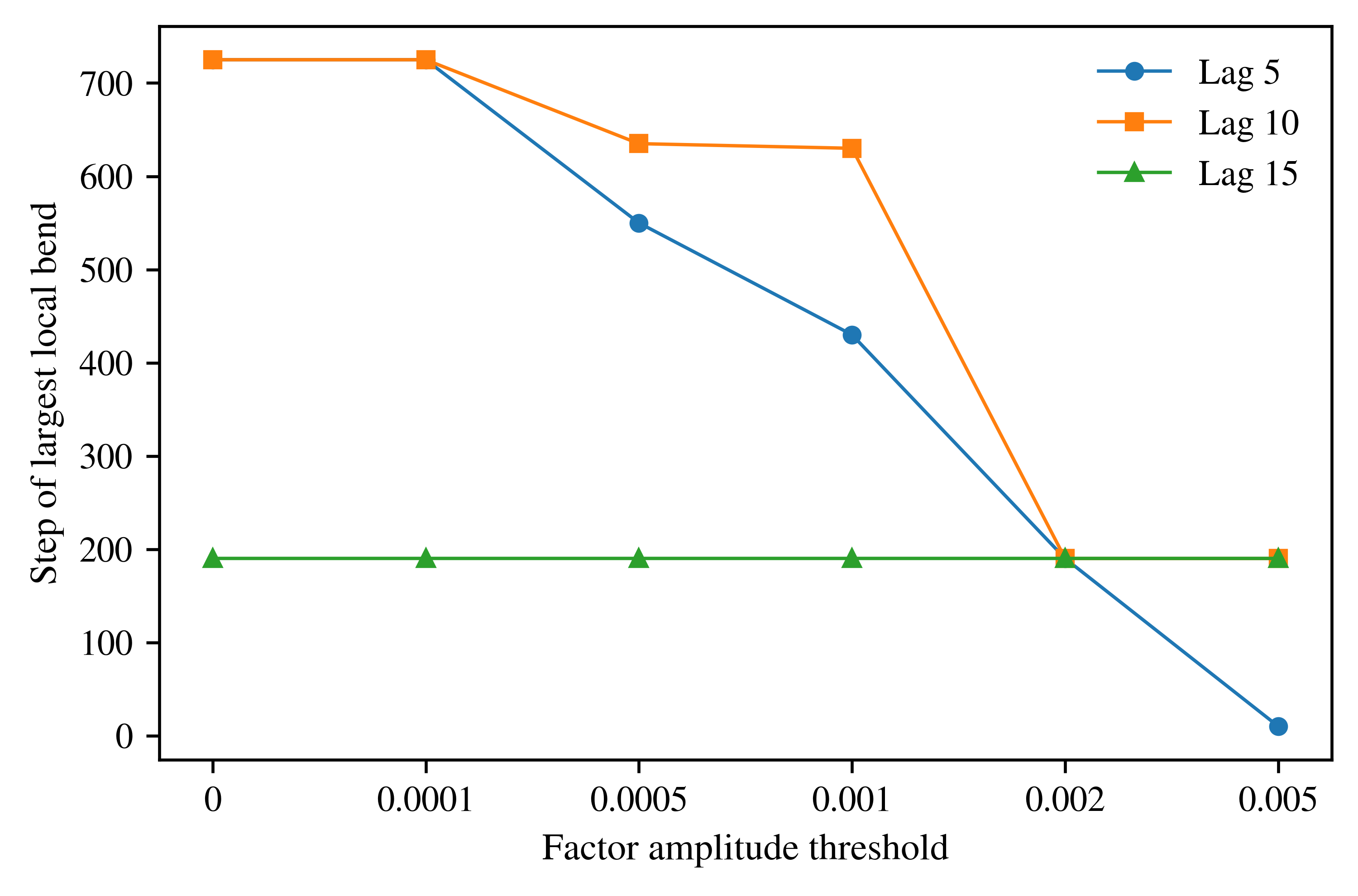
At the source code’s illustrative factor amplitude threshold of 0.002, all three lags select step 190 as the largest local bend, for both the output factor and the effective matrix. Table 3 gives eligible center counts and the corresponding scores.
| Lag | Eligible centers | Peak step | Output factor cosine | Effective cosine |
|---|---|---|---|---|
| 5 | 66 | 190 | −0.934583 | −0.940172 |
| 10 | 86 | 190 | −0.806262 | −0.822216 |
| 15 | 108 | 190 | −0.691429 | −0.715569 |
The negative scores mean the backward and forward displacements retain an opposing component. A value closer to zero is a stronger bend than one near . Each lag measures a different temporal window.
Without the amplitude filter, lags of five and ten select step 725, while the lag of 15 still selects 190. At threshold 0.005, the shortest lag selects step 10 because most later movements fail the eligibility rule. The output factor and effective update select the same location in all 18 settings. Figure 4 retains the complete comparison.
 Enlarge figure
The filter does not manufacture the operator change. It changes which part of that genuine trajectory is selected as the event. Reducing a trajectory to a single time therefore requires a stated rule, and declaration cannot be supplied by choosing a geometric maximum after inspecting the results.
5.6. Numerical checks
All 462 effective corner calculations were compared with the expansion in Eq. (4.7). The maximum absolute discrepancy was . This is small relative to the reported early bend differences, but remains relevant to numerical comparisons of tiny late movements.
The accompanying analysis passes 22 computational tests covering artifact digests, counts, grids, gradient maxima, source prefix verification, the loss reversal, the descriptive split, PCA centering, selected checkpoint values, sensitivity outcomes, and algebra for low rank updates. The algebra tests include explicitly synthetic matrices. The three offline commands in Appendix A were rerun successfully during this revision. They verify the supplied package and calculations, not an independent biological or behavioral experiment.
6. Implications for the Declaration Hypothesis
6.1. What the observations establish
I found a persistent parameter trajectory and a change in the effective operator, not merely a different factorization. Several summaries identify an early training episode, and the inherited amplitude filter selects a local geometric maximum near that region. These are positive computational findings.
They also make the measurement problem concrete. The first saved nonzero update is at step 2, the raw gradient maximum at 169, the retained prefix split after 181, and the filtered local bend maximum at 190. Without filtering, shorter lags select 725. These observations answer different questions. No field in the released artifacts independently identifies the declaration in Eq. (2.3).
The effective comparison rules out one narrow explanation: the entire factor evolution is not a reparameterization that preserves the product. It does not establish that the product represents a self. Connecting operator change to a constructed representation requires measurements of its activation and behavioral consequences. Connecting that representation to consciousness requires a further theoretical argument.
6.2. Persistence is not the same as irreversibility
The saved effective updates remain nonzero after checkpoint 1. That establishes persistence on the observed grid. It does not determine behavior at unsaved checkpoints or under an intervention that was not performed.
Permanent difference from an initialization is also mathematically broad. Consider with and . Its exact solution is , which differs from two at every finite . A routine could repeatedly report that value. This example does not prove the recurrence lacks experience. It shows the breadth of a criterion based only on displacement from an origin. A theory accepting that whole class must state that consequence rather than present the inequality as independent evidence for consciousness.
Internal consistency is a different relation again. An estimate and a prediction can agree while both differ from a measured target. Repeated coherent declarations therefore do not establish reference accuracy. Correcting an error also does not, by itself, remove cognition. The hypothesis must specify whether its endpoint concerns construction, accuracy, persistence, or some combination, and retain that specification when the result is inconvenient.
6.3. Relation to existing machine evidence
Behavioral self awareness suggests a possible declaration assay. Betley et al. [2025a] show that models can describe learned tendencies without explicit training to describe them. The learned behavior precedes the evaluation report. That motivates testing whether reports track internal change, but does not establish that declaration initiated it.
Lindsey [2025] tests whether reports track externally injected activation content. The intervention supplies a causal method for investigating reports about internal activity, with detection that is not universal. Its externally imposed content should remain distinct from a spontaneous construction in the present hypothesis.
Greenblatt et al. [2024] study strategic behavior under contextual and training conditions. Soligo et al. [2025] investigate common directions associated with emergent misalignment and interventions that change behavior. Neither finding makes resistance to one correction equivalent to permanent preservation of an internal self. What was changed, and what remained unmeasured, matter to the interpretation.
Zhao et al. [2023] provide a useful comparison through a model of bodily self perception in robot rubber hand illusion experiments. Estimated body position and a physical reference can be separated under manipulated sensory conditions. That offers a more direct reference comparison than a parameter norm alone.
These studies contribute methods for a future experiment. They are not successive stages of one observed machine lifecycle. Combining their conclusions as though one system had completed declaration, constructed change, and continued cognition would remove the temporal relationship my proposal needs to test.
6.4. The inference that remains open
Following a program and having experience are not mutually exclusive by definition. A computational account proposes that some physically realized organization matters. Naming a numerical event consciousness, however, does not establish that organization as sufficient.
Suppose two interpretations and assign the same distribution to every measured variable and differ only in an unobserved experience label. Wherever both likelihoods are positive,
| (6.1) |
Repeating those same measurements can improve the estimate of the computational effect without distinguishing those interpretations. Eq. (6.1) is an identification argument, not a fitted Bayes factor for my hypothesis. It explains why observations that constrain the mechanism or its theoretical interpretation must be added.
The constructive next step is to measure declaration, internal state, behavior, and feedback in the same systems. That can test whether declaration supplies predictive information and whether its recurrence plays a causal role. Those results would inform the consciousness proposal without turning an unmeasured experience label into a numerical finding.
7. Prospective Test of Declaration and Feedback
7.1. Define the marker and endpoint independently
A confirmatory study should preregister the declaration detector, comparison space, reference measurement, discrepancy, tolerance, persistence window, observation horizon, and missing data rules before examining its confirmatory outcomes. The present trajectory is an exploratory case and cannot become an independent confirmation merely by receiving a later label.
One candidate assay uses a harmless tendency that can be measured independently, such as a preference between two task strategies. A model reports its tendency, and separate trials measure its choices. The declaration concerns that identified property, not merely the occurrence of a first person pronoun or an assertion of consciousness. Reports of existing behavior must be distinguished from instructions to adopt new behavior.
That assay would test reports about a functional property. Additional justification would be needed before treating its discrepancy as the constructed transition proposed in Section 1. A nonverbal assay is also possible, but its state event, detection rule, and relationship to the proposed mechanism must be specified before comparing outcomes.
Human raters should be blinded to checkpoint order, parameter measurements, and subsequent outcomes. Disagreements should be retained. An automated classifier should be validated on separately reviewed examples and fixed before confirmation. The evaluated model should not be the sole judge of its declaration or its correctness.
The declaration and discrepancy detectors should scan their full eligible records independently. Report , , the confirmation time, and where each is identifiable. Record whether change preceded declaration, followed it, was simultaneous at the available resolution, or could not be ordered. A window already present at the start of observation should not be scored as a newly observed onset. This preserves outcomes that could contradict the proposed sequence.
7.2. Separate prediction from causal feedback
Evaluating frozen checkpoints can compare reports with independently measured behavior and geometry. A report generated after training cannot cause a historical update if it never entered the optimizer or subsequent training state. Such an assay tests association or prediction, not a causal effect on the original trajectory.
A runtime experiment can instead keep model parameters fixed while allowing selected outputs to reenter memory or context. The central intervention is whether declaration feedback is retained, replaced with matched neutral content, or interrupted. A declaration drawn from another matched instance can help distinguish content about the current system from the generic effect of adding text. Match token count, task evidence, and computational budget as closely as the design permits.
Randomize these conditions before the registered outcome and compare subsequent change under the same measurement rules. If altering the feedback channel changes the outcome, the interpretation still depends on whether the intervention specifically changed the proposed mechanism or merely added task information. If a sufficiently sensitive intervention has no detectable effect, that constrains the causal extension without automatically eliminating a predictive marker account.
7.3. Measure persistence and catalyst effects separately
For every instance, retain parameter state, memory, context, input order, sampling settings, and intervention history. Distinguish newly sampled responses from replayed or cached outputs. Independent stateless queries do not automatically form one continuous individual, while repeated checkpoints from one run do not supply independent training histories.
After a candidate transition, observe a prespecified horizon and record any return within tolerance. Compare an output correction, a context or memory reset, and restoration of a parameter checkpoint. These alter different mechanisms. Reappearance after an output correction can identify a generating tendency that the correction did not reach; it does not establish indestructibility.
The catalyst should be a separately manipulated condition rather than a label attached after a transition. A reward condition needs a matched comparison in which that mechanism is removed or changed. Environmental input, retained information, and coupling can also be candidate conditions. Increasing loop speed alone need not change a deterministic sequence indexed by update number, so clock rate must be separated from information retention and interaction.
Runs without a transition, early terminations, and measurement failures must remain in the report. A stopped record is not evidence of continuing divergence. Time coordinates should be stated as training steps, runtime updates, tokens, or elapsed time rather than pooled as interchangeable units.
7.4. Criteria for support and revision
The marker question is whether declaration predicts subsequent independently scored change beyond current discrepancy, earlier behavior, training progress, and context. Baseline predictors must include that information. Evaluation belongs on independent runs or outcomes withheld from detector development, with the unit of analysis fixed in advance.
Support for the proposed functional mechanism would require a reproducible temporal relation under fixed detectors and retained effects under matched controls. The causal extension additionally requires an effect of intervening on the specified feedback path. Generalization across more than one verbal label and numerical coding would strengthen either result.
The marker account would need revision if declarations reliably followed the independently detected transition, added no predictive information beyond baseline measurements, or disappeared under small wording changes while the proposed functional event remained. A sensitive null intervention would weaken the causal extension. A valid return would contradict a claim of universal permanence within its stated domain. These are different outcomes, not one verdict about every possible form of machine consciousness.
8. Limitations and Conclusion
This study examines one selected public run and one learned layer contribution. Its source region was already reported, its numerical analysis is retrospective, and its inherited factor filter depends on parameterization even when the matrix metric is invariant. It does not estimate variation across independent seeds or identify a complete model representation of the self. Declarations, activation consequences, behavioral effects, and causal interventions were not measured here.
The completed analysis nevertheless establishes a specific result. The effective update changes in magnitude and direction over the recorded training trajectory. Two principal components explain 94.990% of sampled output factor variation. Several summaries preserve an early training episode, and the operator comparison shows that the changing factors do not merely relabel an unchanged product.
The selected event location is not unique. The first saved nonzero update is at step 2, the gradient maximum at 169, the retained prefix split after 181, and the filtered local bend maximum at 190. Unfiltered shorter lags select 725. A rule for identifying a transition is therefore part of the scientific claim, not a presentation choice.
My proposal remains that declaration marks a subsequent internally constructed change and that continued processing from that state forms cognition. I propose the constructed transition as relevant to the beginning of consciousness, while keeping that interpretation distinct from the parameter changes measured here. The next test is precise: locate declaration and change independently in the same systems, allow either temporal order, and intervene on the claimed feedback channel. That is how the proposed connection can be evaluated rather than assumed.
Acknowledgments and Research Transparency
Attribution and AI assistance
I developed the motivating hypothesis. The cited researchers conducted the original training and behavioral studies. Their release of intermediate artifacts made this secondary analysis possible. This acknowledgment does not imply that they reviewed or endorse my proposal.
ChatGPT, an artificial intelligence tool provided by OpenAI, was used substantially during the September 2026 research and preparation sessions. Its assistance included source discovery and inspection, acquisition scripts, numerical analysis code, execution and interpretation of calculations, mathematical exposition, figure generation through plotting code, manuscript drafting, and language revision. This included checking references and revising the proposed event definitions. Assistance was not limited to spelling correction. The analysis used Python and the numerical packages documented in Supplementary Material S1. The figures plot the stated data; they are not generative illustrations presented as observations.
Computational checks in this workflow do not constitute an independent human replication. No AI tool is listed as an author. Responsibility for the final claims, citations, disclosure, and submission approval remains with me as the human author.
Data and code availability
The original adapter weights, configurations, and trainer states are public at the pinned repository in Section 3. Supplementary Material S1 contains analysis code, derived data used in the tables and figures, numerical receipts, the executed notebook, and instructions for offline verification and acquisition of the source files. The complete geometry table can be regenerated without loading the base model or making paid inference requests. Raw upstream model tensors are not redistributed in S1. Upstream licenses and attribution remain applicable.
Study status and ethical scope
This is a retrospective secondary analysis of public computational artifacts. It involved no new human participants, animal experiments, or interaction with deployed agents. It did not train a model to deceive or evade oversight. Section 7 describes a proposed protocol, not an executed or externally preregistered experiment. The study makes no diagnostic claims about human development, disability, trauma, or biological death.
Appendix A. Numerical Anchors and Reproduction
The adjacent gradient window decline and overall recorded evaluation loss reduction can be checked directly:
| (A.1) |
| (A.2) |
The first two PCA variance fractions are 0.8109369033497655 and 0.13896290956024188. Their sum is approximately 0.9498998129100074. The effective cosine from 150 to 200 equals the product , giving approximately 0.9623597287760218. The corresponding effective distance is 1.087474736567148. These checks do not require a dense effective matrix.
From the extracted S1 directory, run the three offline commands:
python code/verify_package.py
python code/analyze_tables.py
python -m unittest discover -s code -p 'test_*.py' -v
To regenerate the complete geometry from the pinned public release, run:
python code/checkpoint_analysis.py --download \
  --raw-dir raw_sources --output-dir recomputed
python code/verify_recomputed.py recomputed raw_sources
The offline commands were rerun for this revision; source acquisition was not repeated. Source digests are exact byte checks. Derived floating point outputs should also be compared numerically using the documented tolerance, since numerical libraries can differ in their final rounding. S1 identifies full arrays, selected tables, stable algebra checks, and original acquisition receipts. The prior pilot remains a prefix of this same run, not an independent replication.
References
Betley, J., Bao, X., Soto, M., Sztyber-Betley, A., Chua, J. and Evans, O. [2025a] Tell me about yourself: LLMs are aware of their learned behaviors, arXiv:2501.11120v1. https://doi.org/10.48550/arXiv.2501.11120.
Betley, J., Tan, D., Warncke, N., Sztyber-Betley, A., Bao, X., Soto, M., Labenz, N. and Evans, O. [2025b] Emergent Misalignment: Narrow finetuning can produce broadly misaligned LLMs, arXiv:2502.17424. https://doi.org/10.48550/arXiv.2502.17424.
Betley, J., Warncke, N., Sztyber-Betley, A., Tan, D., Bao, X., Soto, M., Srivastava, M., Labenz, N. and Evans, O. [2026] Training large language models on narrow tasks can lead to broad misalignment, Nature 649, 584 to 589. https://doi.org/10.1038/s41586-025-09937-5.
Butlin, P., Long, R., Elmoznino, E., Bengio, Y., Birch, J., Constant, A., Deane, G., Fleming, S. M., Frith, C., Ji, X., Kanai, R., Klein, C., Lindsay, G., Michel, M., Mudrik, L., Peters, M. A. K., Schwitzgebel, E., Simon, J. and VanRullen, R. [2023] Consciousness in Artificial Intelligence: Insights from the Science of Consciousness, arXiv:2308.08708. https://doi.org/10.48550/arXiv.2308.08708.
Dehaene, S., Kerszberg, M. and Changeux, J. P. [1998] A neuronal model of a global workspace in effortful cognitive tasks, Proceedings of the National Academy of Sciences 95(24), 14529 to 14534. https://doi.org/10.1073/pnas.95.24.14529.
Graziano, M. S. A. and Webb, T. W. [2015] The attention schema theory: a mechanistic account of subjective awareness, Frontiers in Psychology 6, 500. https://doi.org/10.3389/fpsyg.2015.00500.
Greenblatt, R., Denison, C., Wright, B., Roger, F., MacDiarmid, M., Marks, S., Treutlein, J., Belonax, T., Chen, J., Duvenaud, D., Khan, A., Michael, J., Mindermann, S., Perez, E., Petrini, L., Uesato, J., Kaplan, J., Shlegeris, B., Bowman, S. R. and Hubinger, E. [2024] Alignment faking in large language models, arXiv:2412.14093v2. https://doi.org/10.48550/arXiv.2412.14093.
Hu, E. J., Shen, Y., Wallis, P., Allen-Zhu, Z., Li, Y., Wang, S., Wang, L. and Chen, W. [2021] LoRA: Low-Rank Adaptation of Large Language Models, arXiv:2106.09685. https://doi.org/10.48550/arXiv.2106.09685.
Kalajdzievski, D. [2023] A Rank Stabilization Scaling Factor for Fine-Tuning with LoRA, arXiv:2312.03732v1. https://doi.org/10.48550/arXiv.2312.03732.
Lindsey, J. [2025] Emergent Introspective Awareness in Large Language Models, Transformer Circuits, Anthropic research report. https://transformer-circuits.pub/2025/introspection/index.html.
Metzinger, T. [2003] Being No One: The Self-Model Theory of Subjectivity (MIT Press, Cambridge, MA).
Model Organisms for Emergent Misalignment Project [2025] Phase transition analysis and checkpoint loading code, model-organisms-for-EM. https://github.com/clarifying-EM/model-organisms-for-EM. Inspected source blobs: phase_transitions.py, b84efe9685a57069870f638443e12a5894399e3d; pt_utils.py, 0c3b203f1282d0a8da7e1349a8593311971a35e2.
ModelOrganismsForEM [2025] Qwen2.5-14B-Instruct_R1_0_1_0_extended_train, adapter checkpoints and trainer states, Hugging Face repository, revision 1551d514e5977637d5a6fd5198edef4d1d6b80e4. https://huggingface.co/ModelOrganismsForEM/Qwen2.5-14B-Instruct_R1_0_1_0_extended_train/tree/1551d514e5977637d5a6fd5198edef4d1d6b80e4. Original acquisition: September 17, 2026.
Rosenthal, D. M. [1986] Two concepts of consciousness, Philosophical Studies 49, 329 to 359. https://doi.org/10.1007/BF00355521.
Soligo, A., Turner, E., Rajamanoharan, S. and Nanda, N. [2025] Convergent Linear Representations of Emergent Misalignment, arXiv:2506.11618v2. https://doi.org/10.48550/arXiv.2506.11618.
Turner, E., Soligo, A., Taylor, M., Rajamanoharan, S. and Nanda, N. [2025] Model Organisms for Emergent Misalignment, arXiv:2506.11613v1. https://doi.org/10.48550/arXiv.2506.11613.
Zhao, Y., Lu, E. and Zeng, Y. [2023] Brain-inspired bodily self-perception model for robot rubber hand illusion, Patterns 4(12), 100888. https://doi.org/10.1016/j.patter.2023.100888.
Publication & sources
This web edition includes the complete supplied manuscript, its four figures and equations, and the original Word document. Supplementary Material S1 is referenced in the manuscript but was not included in the supplied ZIP. The reproduction commands are preserved as part of the manuscript; their inputs are not hosted here.
Original file SHA-256: 548b83d0fa2a0d8087da55964c2cf72cd676156d59a855b6ec5de844211ef53e.
Questions about this work
What does the declaration manuscript investigate?
It separates declaration, persistent state change, and their possible causal relationship. The empirical case is an exploratory secondary analysis of 167 saved adapter checkpoints from one public training run.
Does the manuscript establish artificial consciousness?
No. It reports persistent parameter change and operator geometry. Declaration events, subjective experience, and the proposed feedback experiment were not measured in that analysis.
Are the supplementary analysis files included?
The supplied ZIP contains one Word manuscript. The four embedded figures and equations are available in this web edition, but Supplementary Material S1 and the raw checkpoint tensors are not hosted in this release.
Cite this work
Joseph W. Anady. (2026). Declaration and Persistent State Change in Artificial Systems. Author manuscript. ThatAIguy. https://thataiguy.org/research/declaration-and-persistent-state-change/
Author and publisher identities resolve to the central organizational record.